Examples

Digital portfolio theory uses mean-reversion risk. Below are examples of mean-reversion risks for several industries. These power spectral densities (PSD) or variance spectrums describe the total variance of the returns of each industry. Variance spectrums have been found to be relatively unchanging over time, or stationary. Digital portfolio theory uses both the variance spectrums and the cross-correlations for each mean-reversion period length. The calendar and non-calendar mean reversions are orthogonal, or independent. This allows an equilibrium market model with separation based on period length. A mean-reversion asset pricing model, and a new model market efficiency based on time intervals is implied. Multiple mean-reversion Betas describe systematic risks for each security

Individually these variance spectrums can be used by investors to make investment decisions based on their holding periods.

(These variance spectrums are computed from the Standard and Poor’s Compustat database of index returns from July 1982 to June 1998. The period is studied extensively and includes the October 1987 stock market crash.)

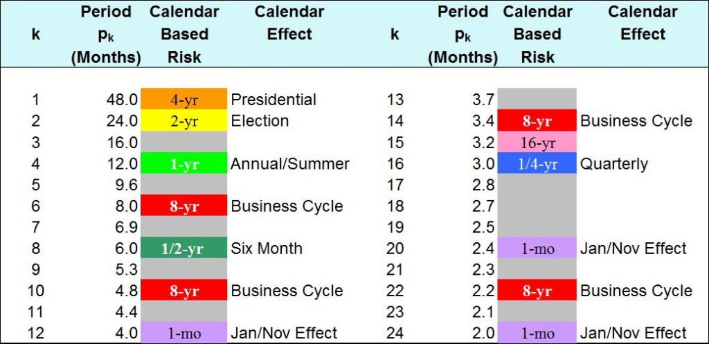
Mean-Reversion Periods

This table will be used to interpret the mean-reversion variance spectrums. It gives all of the mean-reversion periods that can be measured using a 48-month signal length. The mean-reversion periods can be separated into calendar and non-calendar lengths. The table also gives known calendar return anomalies that have been documented by researchers. These calendar anomalies can result in higher mean-reversion risks. If all of the 24 mean-reversion risks are equal the process is a random walk and there is no mean-reversion. If a mean-reversion period has higher risk, it means that the return process has more mean-reversion at that period length. This table is constructed using know calendar effects and their corresponding mean-reversion risk. See Pure Calendar Effects below.

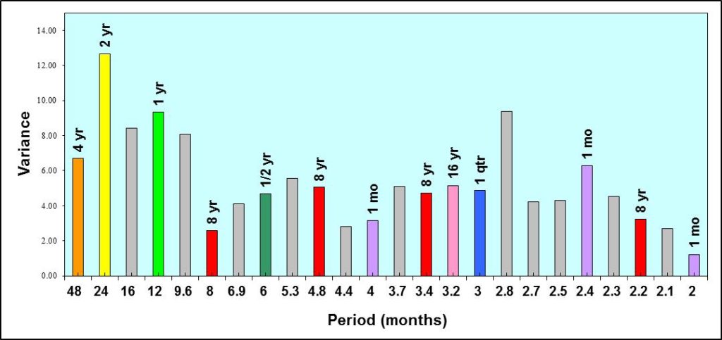
Electronics (Instrumentation) – 500

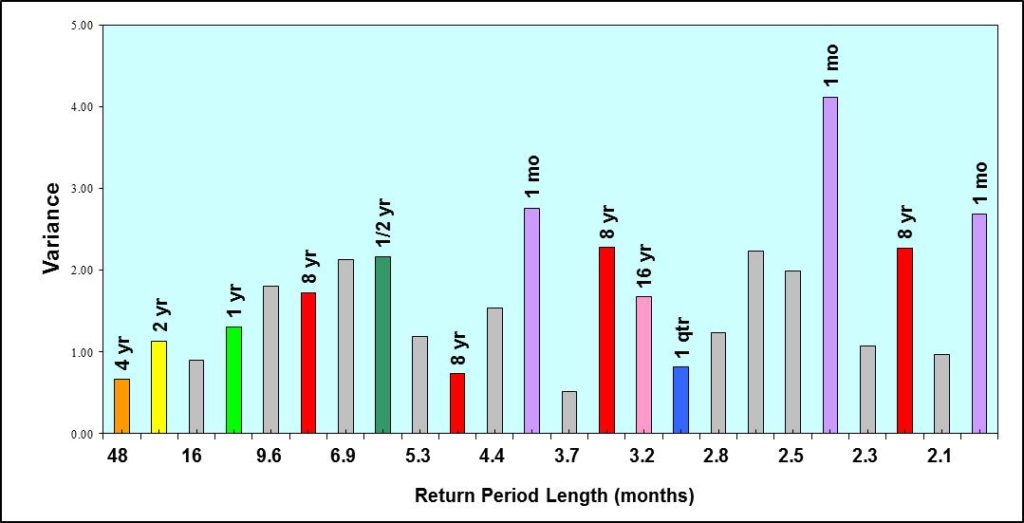
This is the variance spectrum of the Electronics (Instrumentation) – 500 Index returns available from Standard & Poor’s Compustat database. You can see that the electronics industry is dominated by 1-year, 16-year, and 8-year mean reversion risk. Investors interested in investing in the electronics industry should be long-term investors with holding periods of 16 years or longer in order to take advantage of the 1-year, 8-year, and 16-year mean reversions in returns.

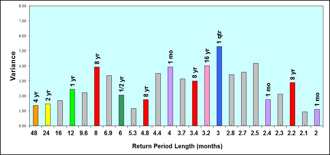
Lodging-Hotels – 500

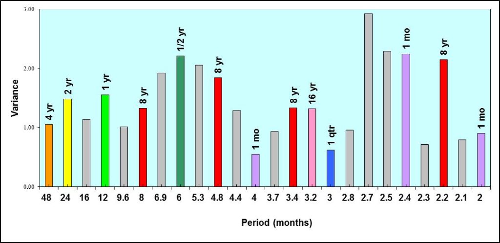
This is the variance spectrum of the Lodging-Hotels- 500 Index returns available from Standard & Poor’s Compustat database. You can see that the lodging and hotels industry is dominated by 2-year mean-reversion risk. Investors interested in buying the lodging-hotels industry should have holding periods of 2 years or longer in order to taking advantage the of 2-year mean-reversion in returns.

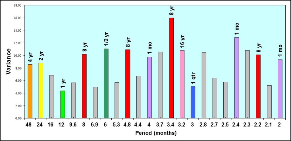
Containers (Metal & Glass) – 500

This is the variance spectrum of the Containers (Metal & Glass) – 500 Index returns available from Standard & Poor’s Compustat database. You can see that the metal and glass container industry is dominated by quarterly mean-reversion risk. Investors interested in buying the containers industry should have holding periods of 3 months or longer in order to take advantage the of quarterly mean-reversion in returns. These investors should be warned that the containers industry also has strong 8-year and 16-year mean-reversion. Therefore containers are also useful for 8 year and 16 year investors. If a 3 month investor believes that containers are in a long term bull market they could remain long. If a 3 month investor believes that containers are in a bear market they could hedge the 8-year and 16-year risk.

Health Care (Medical Products) – 500

This is the variance spectrum of the Health Care (Medical Products) – 500 Index returns available from Standard & Poor’s Compustat database. You can see that the medical products industry is dominated by 4-year and 6-month mean-reversion risk. In addition the strong 2.4-month mean-reversion may indicate a January, or November effect. Investors interested in buying the containers industry should have holding periods of 4 years or longer in order to take advantage the of 4-year and 6-month mean-reversion in returns. These investors should be careful when buying the health care industry to avoid getting caught at the wrong time in a January, or November like effect.

Aerospace/Defense – 500

This is the variance spectrum of the Aerospace/Defense – 500 Index returns available from Standard & Poor’s Compustat database. You can see that the aerospace and defense industry is dominated by 6-month mean-reversion risk. Investors interested in buying the aerospace and defense industry should have holding periods of 6 months or longer in order to taking advantage the of 6-month mean-reversion in returns.

Gold & Precious Metals Mining – 500

This is the variance spectrum of the Gold & Precious Metals Mining – 500 Index returns available from Standard & Poor’s Compustat database. You can see that the gold and precious metals mining industry is dominated by 8-year mean-reversion risk. Investors interested in buying the gold and precious metals mining industry should have holding periods of 8 years or longer in order to taking advantage the of 8-year mean-reversion in returns. The gold and precious metals mining industry also has a January, or November like effect as evidenced by the high 2.4-month mean-reversion risk.

Oil (International Integrated) – 500

This is the variance spectrum of the Oil (International Integrated) – 500 Index returns available from Standard & Poor’s Compustat database. You can see that the international integrated oil industry is dominated by a January or November like effect. Investors should be careful when investing in the oil industry to avoid getting caught buying at the high point in a January, or November like mean-reversion.

S&P 500 COMPOSITE

This is the variance spectrum of the S&P 500 COMPOSITE Index returns available from Standard & Poor’s Compustat database. Note that the S&P 500 has a lower level of variance than any of the other industries. You can see that the S&P 500 is dominated by 6-month, and 8-year mean-reversion risk, and also has a strong January, or November like effect. In addition the S&P 500 has a very high level of noise evidenced by the high 2.7-month mean-reversion risk. This strong noise variance may make the S&P 500 look like a random walk in time domain tests.

Digital portfolio theory uses mean-reversion risk. The mean-reversion risk variance spectrum is composed of calendar and non-calendar length periods. The mean-reversion risk of a particular calendar length is generated by returns that have periodic return changes that occur at that particular calendar length period. For example, 1-year mean-reversion risk is the result of a return time series pattern that has only annual return variation.

January Effect

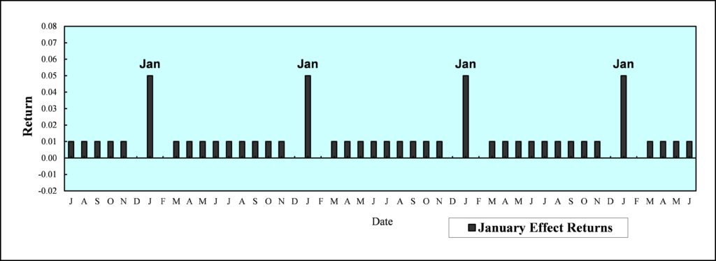
We can construct a hypothetical January effect based on a large number of studies. A January effect is also found in November so the mean-reversion risk of the November effect will be very much the same as the mean-reversion risk of the January effect. The chart shows a hypothetical January effect (or November effect). January has very high return with low return the month before and the month after. In the remainder of the year the monthly returns are flat. The January effect is the strongest calendar effect.

January Effect Mean-Reversion Risk

By taking the Fourier transform of this time series we find the corresponding risk associated with the January effect. The Fourier transform give the variance spectrum or power spectral density. This gives us a signature, or signal of mean-reversion risk that is producing the January effect. The chart shows the mean-reversion risk of the January effect. This is the risk of a monthly effect; it may be produced in the month of January, or in November, or any other month. The mean-reversion risk spectrum described the risk of a monthly effect. It has a distinct signature. Since the monthly effect risk cannot be directly measured with monthly returns and a 48-month signal, the risk (or power) is found in 2-month, 2.4-month, quarterly, 4-month, 6-month and yearly mean-reversion risk.

Quarterly Effect

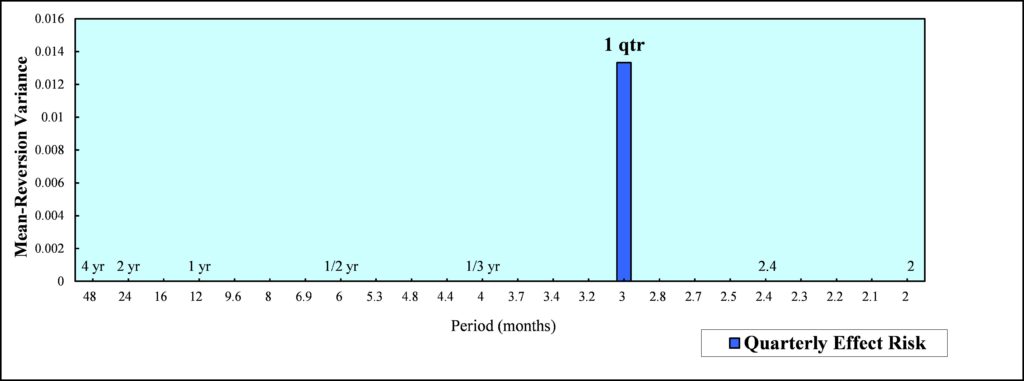
We can construct a hypothetical Quarterly effect based on empirical studies. The quarterly effect has high return in the first month of the quarter and lower returns in the next two months. The chart shows a hypothetical Quarterly effect.

Quarterly Effect Mean-Reversion Risk

By taking the Fourier transform of this time series we find the corresponding risk associated with the Quarterly effect. The Fourier transform give the variance spectrum or power spectral density. This gives us a signature, or signal of mean-reversion risk that is producing the Quarterly effect. The chart shows the mean-reversion risk of the Quarterly effect. Notice that all of the mean-reversion risk or variance is at the quarterly or 3-month period. Since a quarterly effect has only 3 month risk it is a pure calendar effect. The mean-reversion risk spectrum described the risk of a quarterly effect.

Summer Effect

We can construct a hypothetical Summer effect based on empirical studies. The Summer effect has higher returns in the summer months.  The highest return is in July. May has low returns followed by slightly high returns in June. August also has high returns but not as high as in July. The chart shows a hypothetical Summer effect. We must remember that the Summer effect does not happen every year. The Summer swoon effect may have returns that are the mirror image of those in the chart with high negative return in July. This will result in mean-reversion risk that is very similar to the Summer effect mean-reversion risk.

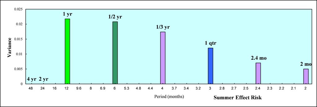
Summer Effect Mean-Reversion Risk

By taking the Fourier transform of this time series we find the corresponding risk associated with the Summer effect. The Fourier transform give the mean-reversion variance spectrum or power spectral density. This gives us a signature, or signal of mean-reversion risk that is producing the Summer effect. The chart shows the mean-reversion risk of the Summer effect. The Summer effect happens annually so it has 1-year mean-reversion risk. It also has strong 6-month mean-reversion risk. The mean-reversion risk spectrum described the risk of a Summer effect.

Presidential Effect

We can construct a hypothetical Presidential effect based on empirical studies. The Presidential effect has the highest returns in the third year of the presidential term.  The fourth year of the presidential term also has higher returns. The first and second year of the presidential term have lower returns. The chart shows a hypothetical Presidential effect. The Presidential effect is strongest for small firms.

Presidential Effect Mean-Reversion Risk

By taking the Fourier transform of this time series we find the corresponding risk associated with the Presidential effect. The Fourier transform give the mean-reversion variance spectrum or power spectral density. This gives us a signature, or signal of mean-reversion risk that is producing the Presidential effect. The chart shows the mean-reversion risk of the Presidential effect. The Presidential effect happens every four years so it has high 4-year mean-reversion risk. It also has stronger 2-year mean-reversion risk. The mean-reversion risk spectrum described the risk of a Presidential effect.

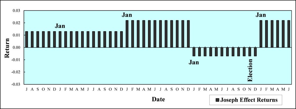
Joseph (8-Year Business Cycle) Effect

We can construct a hypothetical Joseph effect also known as the business cycle based on empirical studies. The Joseph effect is an 8-year effect named after biblical stories. In the business cycle we expect 7 years of positive returns and one year of negative returns. Seven years of feast and one year of famine. The Joseph effect or 8-year effect has high returns in the year before the recession, negative returns for one year during the recession, and high returns for a year after the recession. The next 5 years have lower positive returns. The chart shows four years of a hypothetical 8-year Joseph effect, the other 4 years are the same as the first year in the chart. The business cycle or Joseph effect is the best know calendar effect.

Joseph (Business Cycle) Effect Mean-Reversion Risk

By taking the Fourier transform of this 8 year time series we find the corresponding risk associated with the Joseph effect. The Fourier transform give the mean-reversion variance spectrum or power spectral density. This gives us a signature, or signal of mean-reversion risk that is producing the Joseph effect. The chart shows the mean-reversion risk of the Joseph effect. Since we are only measuring a 4-year signal length, the 8-year mean reversion risk of the Joseph effect or business cycle is reflected in 4-year and 2-year mean-reversion risk, as well as in 8-month, 4.8-month, 3.4-month, and 2.2-month mean-reversion risk. The mean-reversion risk spectrum described the risk of a Joseph effect.