Company Profile
Portfolio Selection Systems is a provider of modeling and decision support for investments. The technology employed is based on Professor Jones’ new theories of portfolio networks, digital portfolio theory, and horizon based capital market equilibrium. The PSS software package offers substantial capability for active and passive investment managers and long-term investors to analyze and optimize their portfolios of assets. The PSS software package enables users to find optimal portfolios of investments using both digital portfolio theory and fundamental analysis with the added dimension of holding period risk. The digital signal processing approach is not available elsewhere. PSS Release 2.0 does not use technical analysis but instead takes advantage of the mean-reversion risk resulting from known calendar effects such as monthly, quarterly, annual, two-year and four-year periods, etc. Optimal portfolios of stocks are selected based on the long-term investor’s purchase date and required holding period.

Dr. C. Kenneth Jones
A Brief History
The portfolio network analysis and digital signal processing model developed in the book and software package are the direct descendant of the Modern Portfolio Theory first developed by Markowitz. The concepts of Digital Portfolio Theory where presented for the first time in a 1983 seminar Portfolio Selection in the Frequency Domain by Professor C. Kenneth Jones and appears in the proceeding of the American Institute of Decision Sciences. The portfolio network model in conjunction with signal processing was the product of Professor Jones’ Ph.D. dissertation published in 1986. In 1992, Ken published his first theoretical textbook Portfolio Management, (McGraw-Hill) presenting portfolio network analysis and deriving the digital portfolio theory model and horizon based asset pricing models. In 1997, Professor Jones published a portfolio selection software package, PSS Rel 2.0 Digital Portfolio Theory, based on the concepts presented in the book. Since the book was published there have been considerable theoretical and empirical advances. In December 2001, the author’s article “Digital Portfolio Theory” appeared in the Journal of Computational Economics. In 2013, Ken’s article “Portfolio Size in Stochastic Portfolio Networks using Digital Portfolio Theory†appeared in the Journal of Mathematical Finance. In 2017 he published a paper titled “Modern Portfolio Theory, Digital Portfolio Theory and Intertemporal Portfolio Choice†in American Journal of Industrial and Business Management.

PSS Rel 2.0 Digital Portfolio Theory
The Evolution of Portfolio Theory
The Markowitz essential insight was to realize that investment analysis in the 1950’s specified that the investor should only be concerned with expected value of return on securities. John Burr Williams and Graham Dodd had not presented any analytic framework for diversification. The value of a portfolio was nothing more than the present value of the future dividends and portfolio diversification was not considered. Diversification has always been a common practice but there was no formal model to reflect the importance of the correlation between assets to effectively diversify. Markowitz’s Modern Portfolio Theory reflected two important characteristics. It incorporated in analytic form a definition of portfolio risk and secondly it showed how this formulation of risk could be used in an optimization model to find efficient portfolios.
Portfolio Network Analysis
Investors have Memory
In 1982, 30 years after Markowitz’s first article, Ken Jones reflected that while Markowitz had added a dimension of risk to portfolio theory there was still a large disparity from what the average investor was doing with regard to their portfolios and the theory. No one can argue about the importance of time to the investor. How many investors have lost or gained fortunes because of timing decisions. If this is the case, what are the components of these timing decisions? Jones distinguished two significant factors missing from portfolio theory. First investors have memory, in the Modern Portfolio Theory model no memory of any past performance or event was utilized other than the estimate of the securities variance and covariance. The Jones insight was to focus on the time dependent characteristics of risk. For example, an investor might observe based on his or her memory “every January since I can remember the small company stocks have done better in January.” The investor remembers that small company stocks have more mean-reversion risk in January. We can use the memory of mean-reversion risk as a rational justification for timing decisions. The Jones insight is that today’s investor, when making a portfolio acquisition or divestiture decision, does not have an analytic measure of this memory nor is there a model to maximize portfolio return that incorporates the memory of mean-reversion risk. While the investment professional must make timing decisions every day, before Digital Portfolio Theory, no quantification of mean-reversion risk memory was available to make such decisions. Instead an assortment of short term technical analysis models, volatility models, and forecasting methods were applied on an ad hoc basis. Professor Jones formulated a definition of mean-reversion risk which allows us to quantify memory in the portfolio theory model. In DPT (digital portfolio theory) there is no forecast of returns, only the memory of mean-reversion risk is used to improve timing decisions. Only mean-reversion risk levels are forecast. You might think of mean-reversion risk as analogous to vibration. Vibrations (risk) can occur at different frequencies, or different mean-reversion lengths. Mean-reversion risks at different frequencies can reinforce each other at regular intervals.

The Holding Period is Missing in Modern Portfolio Theory
The second important missing factor of the single period portfolio decision is how the purchase date and holding period of the portfolio interacts with mean-reversion memory. If it is September and I expect to make a decision to buy a portfolio and hold it for six months, how can the memory of recent and distant past mean-reversion risk levels be quantified and applied? For example, an investor may remember that a particular investment has had downturns in October. In addition to the investor’s October memory, there are in fact many other memory characteristics of a security that may be important even though the investor’s personal memory may not have taken notice. There are multiple mean-reversion risk measures at regular economically significant periods of time. These periods of time are harmonic so the mean-reversion risks are measured at harmonic periods of time. Stock market history does not repeat itself, stock market history rhymes. Rhyming means that the time intervals between risk producing cycles are fixed. This results in multiple harmonic mean-reversion risk levels. For example, in a quarterly time period a particular investment’s mean reverting return pattern may not match the previous quarter, but the level of quarterly mean-reversion risk does match (rhymes). The second moment (variance) is stationary.
For example, you may remember that for a particular investment the first two years of the presidential term has had lower returns than the last two years. The greater the difference between the low returns and the high returns (or prices), the higher the 4-year mean-reversion risk. A particular investment may have more or less sensitivity to the 4-year presidential cycle and therefore more or less 4-year mean-reversion risk. The presidential cycle will induce more or less 4-year mean reversion risk as compared to, for example, a 3-year period. In an economy based on 5-year planning horizons, 4-year risk will not play a significant role as it does in the US economy.
For example, the US health care industry has very high levels of 4-year mean-reversion risk. You can see the mean-reversion risk spectrum of the health industry in Examples. The investor may not remember the sensitivity of a particular investment to the presidential term, but if he or she has a portfolio selection model that measures mean-reversion risk levels, the investor can profit from this knowledge. While past experience is no guarantee of future performance this does not mean we should pretend that our memories of mean-reversion risk levels are irrelevant to our current decision. This was essentially the idea used in MPT and the inter-temporal portfolio choice models since they ignore mean-reversion risks. This was the state of portfolio theory when Jones set about examining the problem as a topic for his Ph.D. dissertation in 1982. The Jones solution was to define mean-reversion risk as a way of quantifying memory, or autocorrelations.
“The world is a harmonious system of contained conflicts†– Alan Watts
The Golden Age of Digital Signal Processing
It happens that one of the newest and most efficient technologies of our time, Digital Signal Processing (DSP) has a solution to this problem of measuring memory. Jones recognized that Digital Signal Processing offers a solution to the quantification of the risk memory for long and short periods. By using long periods (four-years or eight-years) of security returns as digital signals, the memory related to harmonic time interval mean-reversion risks can be accurately measured and incorporated into the portfolio theory model. This new Digital Portfolio Theory (DPT) not only remembers mean-reversions that happened on an annual basis but also remembers the risk from events that occurred on quarterly, six month, 2-year and 4-year ( and even 8-year) bases. In addition, the Digital Portfolio Theory model remembers the effects of events on risks that were not related to regular calendar, or seasonal events. Jones proposed that this non-calendar memory is unrelated to regular time intervals and therefore cannot be used to benefit timing decisions. Markowitz’s Modern Portfolio Theory added a dimension of risk to the return maximization problem that allowed the diversification decision to be quantified. Jones’ Digital Portfolio Theory is a mathematical model that adds the dimensions of memory measured by mean-reversion risks. The Digital Portfolio Theory model offers a rational framework for basing portfolio decisions that are dependent on the point in time and on the holding period of the investor.
The Father of the Digital Age of Finance
If Markowitz is the father of Modern Portfolio Theory, Jones is the father of Digital Portfolio Theory. As Modern Portfolio Theory suggested the CAPM, an equilibrium pricing relationship for all assets based on a linear relation to their betas. Digital Portfolio Theory also implies an equilibrium model based on a linear relationship to multiple mean-reversion betas at multiple periods lengths. This model is concisely presented in Dr. Jones’ 1992 textbook and these calendar Betas are used in the Portfolio Selection System software package available at portfolionetworks.com.
Milton Friedman Rejected the Field of Operations Research
The economist Milton Friedman’s objected that the Markowitz, Modern Portfolio Theory model was “not math, it’s not economics, and its not even business administration”. Friedman’s criticism also implicated Koopmans and the field of linear programming and operations research. This comment has been repeated to Professor Jones many times and continues to this day. Initially Modern Portfolio Theory generated relatively little interest. In fact the portfolio theory of Markowitz was not taught in graduate courses until the late 60’s and then only at a few select universities. One of the biggest drawbacks of Modern Portfolio Theory was that it required a quadratic programming solution. The Markowitz model contained a large number of nonlinear terms so that specialized software was required to find the recommended portfolio. Today practical commercially available software to find the Markowitz efficient frontier from large universes is available to institutional investors but not to the average investor. Dr. Jones has made the new Digital Portfolio Theory financial optimization software PSS Rel 2.0 available to the average investor. Digital Portfolio Theory unlike Modern Portfolio Theory is a completely linear model that maximizes return subject to multiple mean-reversion risk constraints. Digital Portfolio Theory does not require a specialized algorithm to find the optimal portfolio. Because Digital Portfolio Theory is linear, additional constraints can be added, the PSS Rel 2.0 software package allows fundamental analysis criterion to be added to the optimization. The stochastic portfolio network optimization model, solved using DPT is linear and can accommodate very large asset and liability universes. The flow in portfolio networks is a monetary flow. The linear DPT model makes it possible to construct and solve for optimal monetary flow in portfolio optimization models that have millions, billions, and possibly trillions of assets and liabilities. Thus economy wide portfolio networks are a real possibility. Ironically Friedman’s monetarists may in the end utilize the Jones stochastic portfolio network model on an economy wide basis.
The Unexpected Consequences of Digital Portfolio Theory
The Jones application of Digital Signal Processing (DSP) to the portfolio theory problem had three unexpected consequences. First, the portfolio optimization problem formulation was no longer nonlinear! Digital Portfolio Theory allows linear programming to be directly employed to find the solution. The investor can easily create his or her own computer model to try many different risk levels. Secondly, Modern Portfolio Theory required a very large number of terms to represent the risk and correlation structure (variance/covariance matrix). The number of terms increases by the square of the size of the security universe in MPT. Digital Portfolio Theory represents the variance, covariance and autocorrelation with a much smaller number of terms that increases linearly with the security universe size. It is therefore much easier to manage large portfolio universes. Finally, Modern Portfolio Theory solutions are often unreliable because estimation error is greatly magnified in the solution process which requires squared portfolio weights. Additionally since MPT uses correlations between assets the significance of correlation estimates is very low. These problems relegate the MPT model primarily to theoretical importance. To correct these estimation error problems Modern Portfolio Theory often requires users to adjust estimates before optimization. DPT does not magnify estimation error in the solution process. DPT gives more clearly focused risk estimates and the solution portfolios are not distorted by estimation error.
The Digital Portfolio Theory PSS 2.0 software package uses the latest small sample Digital Signal Processing methods currently being employed in speech recognition and other applications. These DSP techniques require a minimum of 16 years of monthly return histories to estimate mean-reversion risks. The new small sample DSP methods utilize multiple overlapping realizations of the security return process and result in more significant estimates of mean-reversion risk inputs to the portfolio optimization model. Since the solution variables in the Digital Portfolio Theory model are linear, more confidence can be placed in the solution portfolios and the distortions commonly associated with Modern Portfolio Theory are greatly reduced.

Dr. Richard Pettway
Early Development of Digital Portfolio Theory
As an MBA student at the University of Florida in 1979, in a Financial Institutions class Professor Richard Pettway suggested that if someone could find a way to solve MPT with a linear solution it would make a substantial contribution. I was also studying nonlinear programming with Professor Ira Horowitz at the University of Florida. I remembered Dr. Pettway’s suggestion when I was working on my Ph.D. at the University of Colorado three years later. While working on an MBA at the University of Florida, I was employed to do empirical financial analysis by Professor Eugene Brigham. I was a natural choice to do computer applications and empirical studies since I had previously worked as a computer programmer at the Chicago Stock Exchange before starting my MBA. One day I was given a deck of computer cards that had recently been obtained from the Wharton School. The program was meant to compute continuous monthly stock betas. Upon examining the program I found that instead of using 60 months of data (the common practice) it was only using only 6 months. “This was a significant lesson for me; empirical work (unlike stock market work) was often of poor quality.â€

Dr. Bruce Golden

Dr. Karen D. Keating
Inspiration for Digital Portfolio Theory
“I came back to Boulder Colorado after a summer break in 1982 I was determined to find a worthwhile topic for my PhD to the University of Colorado. I had taken a course from Professor Fred Glover who was interested in using optimization networks to formulate and solve optimization problems, I was impressed by the graphic representation of optimization and I could see that it held potential in many fields. I went to Fred’s office to ask about dissertation ideas. Fred’s office was piled high with academic papers. Many researchers sent Fred their papers for comment. I told Professor Glover of my interest in finance and asked if he could make any suggestions. Fred had recently received a working paper by Bruce Golden and Karen D. Keating at the University of Maryland. In this paper the authors presented a framework for representing the portfolio problem using network optimization. Of course their models did not incorporate uncertainty. They were purely graphic ways to formulated deterministic financial flow models that could be solved with Linear Programming. Fred gave me this paper along with several other papers. I had just returned to Boulder Colorado for the fall semester at the University of Colorado. I had not found a place to live for the academic year and I was living in a campground in a tent with my girlfriend. I remember sitting at a picnic table next to a lake and looking through the papers Fred has given me. Reading Golden and Keating’s network representation of portfolios, I suddenly remember one of my favorite courses at the University of Michigan when I was undergraduate engineering student. I distinctly remembered R. K. Brown’s famous course in Circuits.
 The electric current flows through wires connected to resistors, capacitors, diodes, and transistors. Circuit analysis employs Kirchhoff’s circuit laws: Kirchhoff’s first law, the current law, is flow conservation. At any node (junction) in an electrical circuit, the sum of currents flowing into that node (where wires meet) is equal to the sum of currents flowing out of that node. Kirchhoff’s second law, the voltage law, is conservation of energy. The sum of the electrical voltage around any closed network is zero. Current and voltage are related using Ohms Law: Current (I) = Voltage (V)/Resistance (R). The voltages may be complex. Kirchhoff’s laws in AC (alternating current) circuits allow current and voltage to have amplitude and phase angle. It is necessary to solve these problems with the mathematics of complex number. Phasor diagrams can be used to find resultant amplitude and phase using vector mathematics.
I remembered how complex arithmetic with real and imaginary numbers is used to find solutions to the current and voltage in AC electric circuits. It was obvious that the monetary flow in portfolio network nodes must satisfy the Kirchhoff’s current law. There must be a conservation of monetary flow at each node in a portfolio network. Suddenly I could see how uncertainly in investment return processes could be described using the same complex arithmetic as in AC circuits. This would allow solutions to incorporate uncertainty in portfolio network analysis. The amplitude would describe the variance or standard deviation. The phase could be unknown. In circuit theory, amplitude and phase are known so the solution is deterministic. It was my background in physics (I was an engineering physics major) that made it clear that a sinusoidal function could be used to describe risk. The uncertainty principle would apply to monetary flows with mean reversions at different frequencies. In physics the position and the velocity of an object cannot both be measured exactly, at the same time. Similarly in monetary flow networks with uncertainty, return and risk cannot both be measured exactly, at any point in time. The phase or time location of a mean reverting return process can be considered uncertain if you know the mean-reversion variances. There is a spectrum of risk similar to the way light can be decomposed in separate colors using a prism. Return is influenced by multiple mean-reversion wavelengths of risk.
Portfolio Selection in the Frequency Domain
The solution to the portfolio network under uncertainty was a visual understanding. I could see multiple sinusoidal waves of risk flowing on the arcs in the portfolio network. Next I derived the mathematical formulation of the classical MPT model in the frequency domain. Off course the correlations must be included. The frequency domain expression for portfolio variance made it possible to include autocorrelation in the portfolio problem as well correlation. I formulated the portfolio variance using phasors (rotating vectors) similar to circuit analysis. The amplitude of the vector represents the standard deviation or risk. The phase angle of the vector is measured relative to the market. I firmly believed that the CAPM was the most important development in finance to that point. The resulting expression I found that portfolio variance was a symmetrical expression with sine and cosine terms. It was still nonlinear; however it was a non-parametric expression that described the total risk and including systematic and unsystematic risk and mean-reversion autocorrelation risk.
Using this expression for portfolio risk in MPT resulted in a much more robust model of portfolio risk since it did not require any assumptions about the distribution of returns and included autocorrelations. (MPT requires a normal distribution of returns and zero autocorrelation). However, this new DPT was still nonlinear but portfolio variance was represented by a more symmetric expression.

Dr. Fred Glover
Having formulated a new DPT problem I went back to Fred’s office to see if he had suggestions on how to solve this nonlinear optimization problem. Dr. Fred Glover is probably the world’s top expert into solving nonlinear optimization using relaxation techniques. When I showed this new digital portfolio theory model to Fred, he patiently explained to me that an optimization with a constraint that contains a sum can be relaxed by using the individual terms of the sum as separate constraints. This was a breakthrough! The sum of the K mean-reversion risks could be made K separate constraints in the optimization problem. Because the expression for the portfolio risk was symmetric, the squared mean-reversion cosine and sine risk terms could to be replaced by their absolute values. These absolute values could be included in the optimization problem as separate constraints. Now risk in units of standard deviation was included in the risk constrained portfolio optimization model with linear constraints. So the linear formulation of DPT contains the solution to the nonlinear MPT variance constrained portfolio selection model because is it a relaxation of MPT. MPT is variance constrained while DPT is a standard deviation constrained model. MPT is quadratic because the variance defined for normally distributed returns in the time domain is quadratic. DPT is linear because the portfolio variance described in the frequency domain is not quadratic but it is symmetric. This symmetry allows the nonlinear non-parametric portfolio variance to be constrained using a set of linear constraints.
DPT is the Natural Formulation of Portfolio Optimization
Now when this set of linear constraints is examined further it was discovered that these linear terms represented sources of systematic risk (cosine terms) and unsystematic risk (sine terms) and that the sum equals total systematic risk and total unsystematic risk for each of the K mean-reversion lengths.
There is a separate set of constrains for each mean-reversion risk component. There are four constraints to control annual mean-reversion risk, or the probably of having 1-year mean reversion. There are four constraints to constrain quarterly mean-reversion risk, etc. The DPT theory problem is linear; the constraints control systematic and unsystematic risk, and control mean-reversion risk for multiple time periods. There is systematic annual mean-reversion risk and there is systematic quarterly mean-reversion risk. But unlike the CAPM there are separate constraints for unsystematic mean-reversion risk, for quarterly, annual, and 2-year periods, etc.
Mean-Reversion Risk and Holding Period
The ability to independently control mean-reversion risks means that holding period plays a significant role in the optimal portfolio. Since autocorrelation information is included, holding period is an important variable in DPT. If we are a one year investor we will hold more quarterly and annual risk. An investor will have a higher expected return and lower risk by increasing risk for mean-reversion risks shorter, or equal to their holding period. Mean-reversions risks longer than the holding period should be reduced. Jones published a paper comparing the DPT model to MPT and to intertemporal portfolio choice, detailing the relationship of MPT and intertemporal portfolio choice to DPT.
Market Equilibrium Models in the Frequency Domain
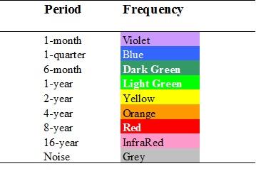
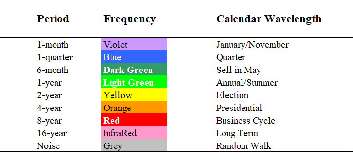
Just as MPT lead to the CAPM, DPT implies a horizon based asset pricing model. The CAPM does not contain separate contribution for mean-reversion risk. The CAPM assumes zero autocorrelations; the holding period was irrelevant to the CAPM investor. DPT implied an autocorrelation CAPM, with separate betas for each mean-reversion risk. There are mean-reversion betas at calendar wavelengths of 1-month, 1-quarter, 6-months, 1-year, 2-years, and 4-years that specify expected returns. In the Jones horizon based asset pricing model, the autocovariance CAPM (A-CAPM) there are annual betas and quarterly betas, etc.,. The holding period of the investor plays a significant role in the asset markets equilibrium price of risk.
There may be many investors with a 1-year holding period; these investors will drive up the price of monthly, quarterly, 6-month, and annual risk. Investors with a 3-month holding period will be interested in increasing quarterly risk, and monthly risk. For the 3-month investor there is no time diversification benefit of holding 6-month, annual, 2-years, or longer mean-reversion risks. These mean-reversion risk contributions will be sold by the quarterly investor. The quarterly investor will have hedging demand for quarterly risk and monthly risk. By increasing quarterly risk, and monthly risk, more 3-month and 1-month mean reversions will influence expected portfolio outcomes. The 3-month investor will have no hedging demands for 4-year, 2-year, 1-year, and 6-month mean-reversion risk, since they are longer than the holding period. So the 3-month investor will reduce these longer-term risks in his or her optimal portfolio. If your portfolio contains only 3-month mean-reversion risk, you will receive the equilibrium level of expected return implied by the quarterly beta. The derivation of both the autocovariance CAPM and the autocorrelation arbitrage pricing theory (A-APT) is found in Jones’s 1992 book “Portfolio Managementâ€.
Empirical Estimation of DPT and the Autocovariance CAPM
Now the new description of Portfolio Network Theory presented in Jones’s book Portfolio Management must be tested empirically. “My Ph.D. program stressed practical results so the model must be empirically tested.†This turned out to be a much more challenging problem than expected. The methodology to estimate mean-reversion risks from time series returns required significant development beyond what the existing state of spectral estimation was capable of achieving. There are many sampling methods and many alternative application of spectral analysis. However, there were no spectral estimation methods specifically designed for estimating financial mean-reversion risks. In fact, because the academic community utilizes time domain models and has very little understanding of frequency domain models, the definition of mean-reversion risk as presented by Jones in his 2011 paper Mean Reversion Risk and the Random Walk Hypothesis did not exist. Mean-reversion risk also presented in this website under Examples can only be defined efficiently in the frequency domain. The overlapping nature of autocorrelations in the time domain means that mean-reversion risk cannot be accurately measured using time domain methods. The vast majority of spectral estimation methods were designed for scientific and engineering applications. The fast Fourier transform (FFT) was a significant benefit in many of these fields. The FFT however, cannot be used in mean-reversion risk estimation. It is necessary to estimate mean-reversion risks and cross-correlations between returns at calendar frequencies (1-month, 3-month, 6-month, 1-year, 2-year and 4-year). The FFT cannot be used for these frequencies.
At the University of Colorado I had complete financial data bases from Compustat and CRSP of security returns histories necessary to compute mean-reversion risks. In 1984 I turned to existing spectral estimation software available for the main frame computer at the University of Colorado. I used multiple spectral estimation software packages. In addition to commonly available time series software and subroutines such a SPSS, SAS, IMSL; I also had STARPAC available from the National Center for Atmospheric Research in Boulder.

Center for Atmospheric Research
I enrolled in every time series and spectral analysis course in the engineering school and in the econometrics department at the University of Colorado. Most of the frequency domain spectral estimation methods used the FFT. The FFT is a computationally efficient method of computing the Fourier transform. Before the development of the personal computer mainframe computers had to be used to estimate Fourier transforms. The limitation of computer power meant that it would take ages to compute a Fourier transform unless the FFT was used. The FFT cannot be used to estimate the DPT model parameters since it can only estimate frequencies at n2 where n=1, 2, 3, etc. So the FFT can compute only frequency such at 1, 4, 9, 16, 25, etc. To estimate the mean-reversion risk levels of DPT we need to estimate frequencies at 2, 3, 6, 12, 24, and 48.
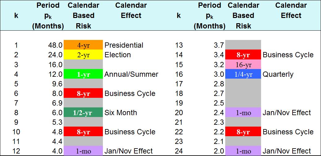
Horizon Risk Levels used in DPT
Calendar Mean-Reversion Risk Levels
To find mean-reversion variances at these frequencies the spectral estimation must compute Fourier transforms directly. Before 1987 this was not a feasible option since it would require more computer time than was realistically practical. There are many questions related to sampling frequency, time series length, spectral windows, overlapping methods, signal lengths, etc. that must be tailored for financial return data. In addition, while returns are available hourly or daily, these periods are difficult to utilize when estimating calendar periods. Only monthly data can be used to find good estimates of the mean-reversion risks used in DPT. DPT is truly a long-term model. It is of no use to the volatility trader and it provides no forecasting of returns. The DSP (digital signal processing) methods used in DPT only estimate levels of mean-reversion risks they make no forecast of the path of returns through time. Mean-reversion risk levels are used by DPT to increase expected portfolio return and reduce portfolio risk for a specific holding period.
For my Ph.D., I decided on a compromise approach using daily data to try to capture the benefits of DPT without finding an exact estimation. Since unlike MPT, DPT can be implemented for large security universes, I used a large number of stocks and I used long time horizons. I began computing complete databases of spectral estimates and using them to find DPT solution portfolios for multiple levels of risk. This required considerable computer resources and it was not long before I was contacted by Ron Melicher the head of the finance department at University of Colorado about my computer usage.

Dr. Ronald Melicher
I explained that it was necessary and to his credit he requested more computer resources on the university’s main frame computer. It was not long before I was single handedly using more computer time than the engineering school. Again Professor Melicher fought for my computer usage and for 2 years I ran large optimization and large spectral estimations every night on the mainframe computer. When I completed my Ph.D. in 1986 the PC (personal computer) was first beginning to appear.
The Application of Digital Signal Processing
Despite considerable effort in my Ph.D., I had not found a satisfactory method for estimating mean-reversion risks needed for DPT. I continued to study spectral estimation of stock returns. Spectral estimation of stock market data was not new; Granger and Morgenstern (1963) Granger and Hatanaka (1964), Jenkins and Watts (1969), Priestley (1981) published books on the subject and hundreds, if not thousands of researcher have attempted to apply spectral estimation to stock market data. Even today, hoping to get rich quick, most universities have a least one student or professor every year who again attempts to use spectral analysis to examine stock prices. Most of these efforts are not useful for capital market theory and end in failure. The common reason for these failures is that spectral estimates are used as a forecasting method for short-term profit rather than as a means for estimating long-term risk. There is further confusion because researchers think the FFT can somehow be applied to economic data. Finally many think that since high frequency data is available such as daily, hourly, or trade-by-trade data that it should provide the best estimates using spectral analysis. All of these assumptions are false and lead to results that do not reflect the underlying calendar length nature of economic processes and their long-term frequencies.
The Jones Vision of Return Dynamics in the Frequency Domain
I realized that the PC was the answer to computing spectral estimations of stock return time series since the PC would not be bound by a mainframe computer budget. I was forced to wait for more PC power. After completing my Ph.D. at the University of Colorado I was ready for some adventure. I became assistant professor of finance at the University of Petroleum and Minerals for four years from 1986 to 1990 in Saudi Arabia. During this time I wrote the theoretical textbook outlining portfolio network analysis and deriving the DPT model and the calendar based CAPM. In this book, Portfolio Management published by McGraw-Hill in 1992, I defined calendar and non-calendar mean-reversion betas. By the time I returned to teach at the University of Florida in 1990-1991, the PC had finally come into its own and I realized that Fourier spectral decomposition software must be written for long-term returns in order to put my portfolio network theory into practice. I began writing my own spectral analysis software programs. At the University of Florida I not only taught International Finance but went back to school in the Electrical Engineering department studying the new field of digital signal process. Many people do not realize that the field of digital signal processing (DSP) originated with the publication of textbooks such as “Signals and Systems†by Oppenheim and Willsky (1983) and “Discrete-Time Signal Processing†by Oppenheim and Schafer (1989). So the field of DSP had only been around for a few years when I returned to engineering school at the University of Florida. These new discrete-time finite length methods were essential to create mean-reversion risk estimates. The power and simplicity of DSP was astonishing. I could see a very big future for the use of DSP in financial theory.
At the same time at the University of Florida, I began studying in the computer science department. I took a computer programming course on how to use spreadsheet macros to write a software package. This was the beginning of the PSS Rel 2.0 DPT software package published in 1997, six years later. I spent all of my time creating accurate DSP software capable of managing long time series stock returns and large securities universes, and capable of finding efficient portfolio optimizations. At is point I had one more resource without which none of my work to that point would have been possible. My father, C Howard Jones was a researcher in frequency domain applications and holds over 40 patients in diverse fields of radio, antennas, high definition television, microwave commutations, and sonar.

C. Howard Jones
My father also did a wide ranging study of the entire electromagnetic spectrum. He outlined all frequency domain applications using electromagnetic radiation. This was presented visually in terms of wavelengths. He created a chart that visualizes the entire range of electromagnetic waves at wavelengths from low frequency electrical power and telephone waves (up to 25 cycles per second) to high frequency cosmic rays, or elementary particles (at .01 milli-angstroms, or 1230 million electron volts). His study and representation of the electromagnetic spectrum remains the state-of-the-art today.
Electromagnetic Spectrum by C. Howard Jones
My thesis was that financial risk itself travels like waves but at lower frequencies than electromagnetic waves. These frequencies are the natural time dimensions of economic events. They are the carriers for long-term risk and correspond to calendar seasonal and cyclical wavelengths. Incredibly this idea is questioned by researchers, whose entire focus is on volatility occurring daily or at even shorter periods. The world of finance is awash with volatility models driven by researcher whose dream is to get rich quick. These researchers see no value in being able to measure long-term mean-reversion risks.
Without my father’s encouragement I could not have pursued the frequency domain field of finance. I described to my father my problem of creating a software package that applied the Fourier transform to find low frequency spectrums of risk in financial returns. With Dad’s help we constructed a computational method for directly computing Fourier transforms for financial frequencies that was particularly well suited to a spreadsheet framework. This became the basis for my spreadsheet software that computed the signal processing mean-reversion variance decomposition used in DPT.
After having used so many spectral estimation programs I was amazed and impressed with the speed and accuracy when the Fourier transform was computed at calendar harmonic frequencies from monthly data using this spreadsheet approach. Commercially available PC software such as IMSL are unable to find these kinds of estimates for long-term financial returns. Now I had a reliable and significant method of finding horizon based risk estimates used in DPT. I went on to test this software using all US stock market data available in the CRSP database. I found in fact, that the hypothesis that calendar mean-reversion risk levels are generated by random walks was false. Financial returns have a distinct calendar mean-reversion risk structure. This study Calendar Based Mean Reversion Risk and Digital Signal Processing (2008) can be downloaded and examples of this calendar risk structure can be found under Examples on this website.
I decided on the publishing a DPT software package because I felt that a space shuttle type approach was required; to lift finance out of the time domain, and to refocus financial researchers obsession with volatility, to a world of long-term risk waves. Markowitz developed an algorithm called the critical line method to find efficient frontier portfolios. However the critical line software was never published by Markowitz as a software package available to researchers or investors. One of the reasons for this is that the portfolios found by MPT are embarrassingly unstable. This was not Markowitz’s fault; it was a problem with the specification of MPT as a quadratic problem that uses stock return correlations. After publishing the software package Portfolio Selection System: Digital Portfolio Theory, I mailed free examination copies to many researchers.
The Slow Acceptance of DPT
The new frequency domain portfolio optimization and horizon dependent market equilibrium models have experienced substantial resistance. The field of finance is still completely focused on linear regression models which have been extended to autoregressive models. These models are not helpful in understanding time interval dependent risk. To make the leap from linear regression to thinking in the frequency domain in terms of mean-reversion risks is asking too much of the financial researcher. The fact that risk could be represented as waves with multiple wave lengths is not consider possible since it is well know that the history of financial returns is random and that mean-reversion risk cannot be measured. In fact mean-reversion risk has never been measured in the time domain because of overlapping period lengths. That is, in order to measure annual risk, how do you remove the effect of six- month and quarterly mean-reversions? In the time domain it is not possible, but in the frequency domain annual mean-reversion risk, six-month mean-reversion risk, and quarterly mean-reversion risk can be measured directly and are separate and independent. It seems that investors are not able to think about long-term risk without becoming confused by short-term volatility. Over ninety percent of the risk faced by investors is long-term risk and correspondingly over ninety percent of the returns are long-term. MPT focuses on less than ten percent of the risk. We are currently in the “age of volatility†in financial theory. How long will it take for the field of finance to move to the golden age of digital signal processing and to the age of long-term risk?
Media Inquiries
Media inquiries for background information or to coordinate interview requests to:
Contact: info@portfolionetworks.com
© Copyright C. Kenneth Jones 2017